Getting started
![]()
![]()
![]()
PauliStrings.jl is a Julia package for many-body quantum simulation with Pauli strings represented as binary integers. It is particularly adapted for low-magic applications, efficiently manipulating local operators, time evolving noisy systems and simulating spin systems on arbitrary geometries. Paper : https://arxiv.org/abs/2410.09654, Python version

Documentation
The documentation is there : https://paulistrings.org
To build the docs :
julia docs/make.jlInstallation
You can install the package using Julia's package manager
using Pkg; Pkg.add("PauliStrings")Or
] add PauliStringsInitializing an operator
Import the library and initialize a operator of 4 qubits
import PauliStrings
H = Operator(4)
Add a Pauli string to the operator
H += "XYZ1"
H += "1YZY"
julia> H
(1.0 - 0.0im) XYZ1
(1.0 - 0.0im) 1YZYAdd a Pauli string with a coefficient
H += -1.2, "XXXZ" # coefficient can be complexAdd a 2-qubit string coupling qubits i and j with X and Y:
H += 2, "X", i, "Y", j # with a coefficient=2
H += "X", i, "Y", j # with a coefficient=1
Add a 1-qubit string:
H += 2, "Z", i # with a coefficient=2
H += "Z", i # with a coefficient=1
H += "S+", i
Supported sites operators are X, Y, Z, Sx=X/2, Sy=Y/2, Sz=Z/2, S+=(X+iY)/2, S-=(X-iY)/2, Pup=(I+Z)/2, Pdown=(I-Z)/2.
Basic Algebra
The Operator type supports the +,-,* operators with other Operators and Numbers:
H3 = H1*H2
H3 = H1+H2
H3 = H1-H2
H3 = H1+2 # adding a scalar is equivalent to adding the unit times the scalar
H = 5*H # multiply operator by a scalar
Trace : LinearAlgebra.tr(H)
Frobenius norm : LinearAlgebra.norm(H)
Conjugate transpose : H'
Number of terms: length(H)
Commutator: commutator(H1, H2). This is much faster than H1*H2-H2*H1
Print and export
print shows a list of terms with coefficients e.g:
julia> println(H)
(10.0 - 0.0im) 1ZZ
(5.0 - 0.0im) 1Z1
(15.0 + 0.0im) XYZ
(5.0 + 0.0im) 1YY
Export a list of strings with coefficients:
coefs, strings = op_to_strings(H)Truncate, Cutoff, Trim, Noise
truncate(H,M) removes Pauli strings longer than M (returns a new Operator) cutoff(H,c) removes Pauli strings with coefficient smaller than c in absolute value (returns a new Operator) trim(H,N) keeps the first N trings with higest weight (returns a new Operator)
add_noise(H,g) adds depolarizing noise that make each strings decay like $e^{gw}$ where $w$ is the length of the string. This is useful when used with trim to keep the number of strings manageable during time evolution.
Time evolution
Time evolution in the Pauli strings basis is commonly referred to as sparse Pauli dynamics, Pauli paths simulation, Pauli propagation or Pauli backpropagation.
The main entry point is evolve(H, O, tspan; method, fout, dissipation, truncation), which integrates O in the Heisenberg picture and saves the value of fout(O) at every time in tspan. Available integrators are RK4(), DOPRI5(), Trotter(), and Exact().
Each save step performs (1) one integrator step, (2) an optional dissipation step (typically depolarizing noise via add_noise), and (3) an optional truncation step (typically trim). The combination of noise and truncation is what makes long-time simulations tractable.
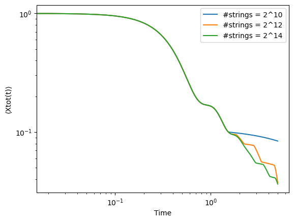
Below we evolve $Z_1$ in a chaotic spin chain and record the autocorrelator $S(t) = \tfrac{1}{2^N}\textup{Tr}\big[Z_1(0) Z_1(t)\big]$ for several truncation levels:
using PauliStrings

function chaotic_chain(N::Int)
    H = Operator(N)
    for j in 1:N
        H += "X", j, "X", mod1(j+1, N)
    end
    for j in 1:N
        H += -1.05, "Z", j
        H +=  0.5,  "X", j
    end
    return H
end

N = 32
H  = chaotic_chain(N)
O0 = Operator(N) + ("Z", 1)
dt = 0.02
times = 0:dt:5

dissipation(O, dt) = add_noise(O, 0.05 * dt)
fout(O) = real(trace_product(O0, O) / 2^N)

for M in [10, 12, 14]
    truncation(o) = trim(o, 2^M)
    res = evolve(H, O0, times;
                 method=RK4(), fout=fout,
                 dissipation=dissipation, truncation=truncation)
    # plot times vs res.history
end
A runnable version is in examples/evolve_chaotic.jl (and examples/evolve_tfim.jl). See the time evolution tutorial for a walkthrough.
Lanczos
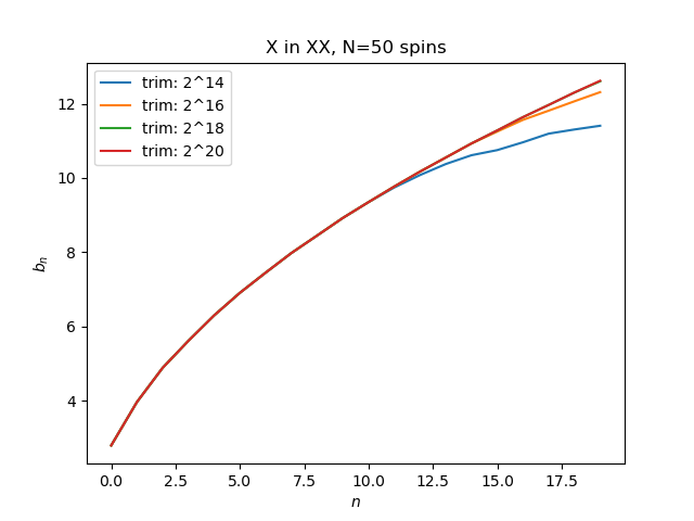
Compute lanczos coefficients
bs = lanczos(H, O, steps, nterms)H : Hamiltonian
O : starting operator
nterms : maximum number of terms in the operator. Used by trim at every step
Results for X in XX from https://journals.aps.org/prx/pdf/10.1103/PhysRevX.9.041017 :
Circuits
The module Circuits provides an easy way to construct and simulate circuits. Construct a Toffoli gate out elementary gates:
using PauliStrings
using PauliStrings.Circuits

function noisy_toffoli()
    c = Circuit(3)
    push!(c, "H", 3)
    push!(c, "CNOT", 2, 3); push!(c, "Noise")
    push!(c, "Tdg", 3)
    push!(c, "CNOT", 1, 3); push!(c, "Noise")
    push!(c, "T", 3)
    push!(c, "CNOT", 2, 3); push!(c, "Noise")
    push!(c, "Tdg", 3)
    push!(c, "CNOT", 1, 3); push!(c, "Noise")
    push!(c, "T", 2)
    push!(c, "T", 3)
    push!(c, "CNOT", 1, 2); push!(c, "Noise")
    push!(c, "H", 3)
    push!(c, "T", 1)
    push!(c, "Tdg", 2)
    push!(c, "CNOT", 1, 2); push!(c, "Noise")
    return c
end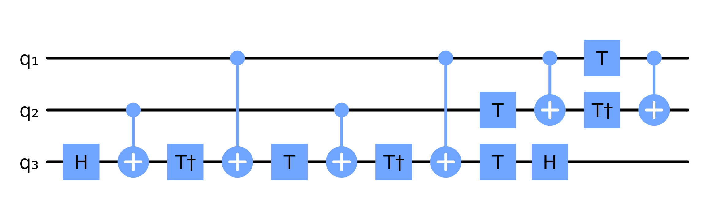
Compute the expectation value $<110|U|111>$:
c = noisy_toffoli()
expect(c, "111", "110")
Contributing, Contact
Contributions are welcome! Feel free to open a pull request if you'd like to contribute code or documentation. For bugs and feature requests, please open an issue. For questions, you can either contact nicolas.loizeau@nbi.ku.dk or start a new discussion in the repository.
Citation
@Article{Loizeau2025,
	title={{Quantum many-body simulations with PauliStrings.jl}},
	author={Nicolas Loizeau and J. Clayton Peacock and Dries Sels},
	journal={SciPost Phys. Codebases},
	pages={54},
	year={2025},
	publisher={SciPost},
	doi={10.21468/SciPostPhysCodeb.54},
	url={https://scipost.org/10.21468/SciPostPhysCodeb.54},
}

@Article{Loizeau2025,
	title={{Codebase release 1.5 for PauliStrings.jl}},
	author={Nicolas Loizeau and J. Clayton Peacock and Dries Sels},
	journal={SciPost Phys. Codebases},
	pages={54-r1.5},
	year={2025},
	publisher={SciPost},
	doi={10.21468/SciPostPhysCodeb.54-r1.5},
	url={https://scipost.org/10.21468/SciPostPhysCodeb.54-r1.5},
}